Diffusion in general is the interpenetration between two and more substances without any chemical reaction. Diffusion
causes the flow rate at which matter moves across a unit area. It is sensitive to the temperature and the viscosity of the medium wherein it occurres. Diffusion
of liquid into another, the transfer of heat or electricity from one point in
space to another, they all are examples of “fluxes” induced by “forces”. These
forces
are gradients of
concentration, differences in temperature, or electrical potential, respectively. For details see Cussler 1997, Kleeman 1920 and Reid et al. 1977. Berthollet
(1803) was the first, who pointed out the analogy between heat flow and
diffusion, when he discussed the mechanism of the dissolution of a salt crystal
in water: “The crystal dissolves, and the removal of the dissolved solute from
its surface may involve pure diffusion, occuring without visible movement of
the solution at a whole, and, in addition, a macroscopic flow of the denser
parts of the solution relative to the lighter parts. Similarly, heat flow by
conduction may be accom- panied by convection;” (cited by Tyrrell 1961).
Fourier
(1822) found that in the case of heat
conduction the flow of heat is in linear relationship to the gradient of
temperature. Five years later it has been shown by Ohm that the electric
current flowing in a conductor was linear to the potential difference between
the ends of the conductor. A simple linear function dominates both flow of heat
and electricity. It was Fick (1855) who assumed upon Berthollet’s analogy that
the force responsible for diffusion is the gradient of concentration, and he
formulated the first and second law of diffusion. This linear
relationship is given by the differential equation (in a one-dimensional
system) J = - (constant) df/dx.
J
represents the transport or flow of heat, matter or electricity in direction x
perpendicular across a reference plane of unity, df/dx is the corresponding
“force” namely gradient of temperature, concentration of dissolved molecules or electrical potential.
And so the flow of heat, molecules and electricity can be written as
J = - k dT / dx (Fourier’s Law) J = - D dC / dx (Fick’s Law)
J = - κ dΨ / dx (Ohm’s Law)
where T, C
and ψ are temperature, concentration and electrical potential, respectively.
and k, D and κ are the corresponding coefficients.
If the
conductor is a uniform bar of lenght L with a cross-section of unity across which
a constant potential (-ΔΨ) is applied than Ohm’s law looks like
I = (- κ/L) (-ΔΨ) = ΔΨ / R,
where R is called the
electrical resistance regulating the electrical current I caused by the
electrical potential ΔΨ.
This
is one of the most frequently used equations on earth.
Coming back
to diffusion of molecules or larger particles it should be mentioned that two
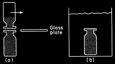
men have been pioneers in this field: Thomas Graham and Adolf Fick. Graham (1829, 1833)
built the first instruments to study the diffusion in gases and liquids, figures 1a,b.
Fig.1a: Graham’s
diffusion tube for gases. This apparatus was used in the best early study of
diffusion. A gas like hydrogen diffuses out through the plug, the tube is
lowered to ensure that there will be no pressure difference.
Fig.1b: Graham’s
diffusion apparatus for liquids. The equipment in (a) is the ancestor of free diffusion
experiments ; that in (b) is a forerunner of the capillary method.
He could show that diffusion in gases was
several thousand times faster than in liquids and he concluded that “the
quantities diffused appear to be closely in propotion to the quantity of salt
in the diffusion solution” Graham (1850 p.6). Here he statet that the diffusion
rate is proportional to the concentration drop.
Adolf Fick
brought the next major advances to modern understanding of diffusion.
He was born in 1829 when
Graham etsablished his first apparatus for gases. His first intention was to
become a mathematician but he has been persuaded by his older brother, a
professor of anatomy, to change to medicine. Major topics in his scientific
life did not depend on diffusion at all, but on general studies of physiology.
He was particularly interested in the function of muscles and in the visual and
thermal functioning of the human body.
It was 1855
when he published his first diffusion paper and introduced it with: “Diffusion
of dissolved material is left completely to the influence of the molecular
forces basic to the same law ... for the spreading of warmth in a conductor and
which is already been applied with such great success to the spreading of
electricity” (Fick 1855, p. 65). In analogy to Fourier’s heat equation he
developed the laws of diffusion. Fick called the quantity D “the constant
depending of the nature of the substances” which we call the diffusion
coefficient.
The
dimension of D is square centimeter divided by time in seconds. The values of D
differ by several magnitudes depending on the state of aggregation.
Some
representative examples of diffusion coefficients:
in gases: CO2 in air D
= 0,14 cm2/sec in liquids: NaCl in water D
= 0,14 • 10-5 cm2/sec glucose
in water D = 0,6 • 10-5 cm2/sec urea
in water D = 1,4 • 10-5 cm2/sec in biomolecular environment: H2O in lipid bilayer D = 3 • 10-10 cm2/sec in metals: carbon
in steel D = 0,14 • 10-12 cm2/sec
Molecules
in liquids or gases are not at rest. They are very rapidly and perpe- tually
moving, colliding with each other and changing speed and directions due to
these collisions.
These
movements are due to thermal energy and are also called thermal noise (Berg 1993, Feynman et al. 1970).
On the
average the kinetic energy of a molecule at absolute temperatur T is kT/2,
where k is Boltzmann’s constant. On the
other side, the kinetic energy of a molecule with mass m and
moving with velocity v
is given by
which
leads to equation
resulting
in
In reality
the velocity is anything but constant in time but fluctuates very rapidly
around this mean value of kT/m. Brackets < > denote the average over time
and
the correct expression therefore is
This kinetic energy is deep-rooted into every particle of any solution and is the cause of various phenomena in it. Random
migration and continuous agitation of very small bodies (bacteria, tiny dust particles or colloids) in
water for instance is caused by a permanent bom- bardment and unbalanced impacts of surrounding water
molecules where the inequality of the momentary collisions on one side to the
other lead to a “jiggling around”. These
movements have been observed soon after the discovery of the light mi- croscope,
especially by its inventor Leeuwenhoek (1632-1723) and some others.
Robert Brown (1773-1858, figure 2) indeed was the first, who discussed this
phenomenon in detail (1828, 1829) during his microscopical investigations on
pollen grains of some flowering plants. Due to his contributions the irregular
motion of small particles in gases and liquids is called the “Brownian
(molecular) motion”.
Fig.2: Robert
Brown in the 3rd and 6th decennium of
the 18th century
This motion
never ceases and can be observed even in liquid inclusions in quartz thousands
of years old. This experience together with the fact that non-viable mineral
objects like dust particles also show these phenomena led Brown – in
contradiction to other scientists in his time – to the conclusion that these
move- ments are not due to any type of animation.
The
Brownian motion is completely irregular in a haphazard fashion and in all
directions. Observations of these movements are mostly performed in the two
dimensional plane. Perrin (1923) was one of the first scientists, who made
extensive investigations on this phenomenon and fig.3 gives an expample of his
data published in Atoms (Die Atome ).
Fig.3: Planar Brownian motion of microscopic particles in two dimensions
In his
capital year 1905 Einstein published a mathematical theory for the explana- tion
of the Brownian motion and deduced a way to use this motion for the
deter- mination of Avogadro’s number. In 1908, the French physicist Jean-Baptiste
Perrin verified these ideas experimen- tally. He did a lot of work on measuring
this quantity and they both provided the evidence for the molecular structure
of matter, which is well-established today. When Brown did his observations in
1827 it was not so!
For his
work Perrin was honoured with the Nobel Prize in 1926.
Upon
Brownian motion a particle moves back and forth but the distance x from the
starting point gradually increases. This spreading out in only one dimension
leads
to the relationship
where <x^2> is the mean-square displacement of particles
in time t. The quantity D characterizes the migration velocity of the particles of a given kind in a
given medium at a given temperature and is our well-known diffusion coefficient.
The
mean-square of the diffusion path of a particle is proportional to the
diffusion time
and the diffusion
coefficient.
The average displacement of a particle is then given by
The time t to migrate along the path x is
For urea in
water we had
This
molecule will walk through a bacterium (width x ~ 0,0001 cm) in
or roughly
half of a millisecond.
It diffuses
a distance of 1 cm (width of a test tube) in t = 36-thousand seconds,
lasting 10 hours.
Eq.7 is valid for each direction in the three dimensional space.
Diffusive displacements in more than one dimension are connected with the
relationship <x^2> = 4Dt in planar and
<x^2>
= 6Dt in cubic dimensions.
diffusion coefficient of DAPI
We will try to derive the diffusion coefficient of DAPI by using the
coefficient of rhodamine B or rhodamine 6G (furthermore refered to as
rhodamine) as one of the reference molecules in fluorescence spectroscopy (Thaer
and Sernetz 1973, Rost 1991, Lakowicz 2006).
A publication of Rigler et al. 1993 on
fluorescence corre- lation spectroscopy has often been cited by refering to the
diffusion coefficient of rhodamine to be 2,8*10^-6 cm^2/sec.
But if one
searches in detail through that paper it will become clear that Rigler solely
did use this value without any reference.
All publications until now were based on
data which have been generated nearly a century ago (Herzog and Polotzky 1914). For details see section “tracing rhodamine”. The diffusion coefficient increases with
temperature and fluidity of the surrounding medium and is proportional to the
square root of the mass of the diffusing molecule (Herzog and Polotzky 1914,
Wawilow 1925, Wilke and Chang 1955, Chapman and Cowling 1970, Cussler 1997).
Assuming the value of 2,8*10^-6 cm^2/sec for rhodamine with a molecular weight
of 479 we calculate - as a first correction - a value for DAPI with molecular
weight of 368
to be 479^1/2
/ 368^1/2 = 1,14 larger. The second correction is based on the fact that the
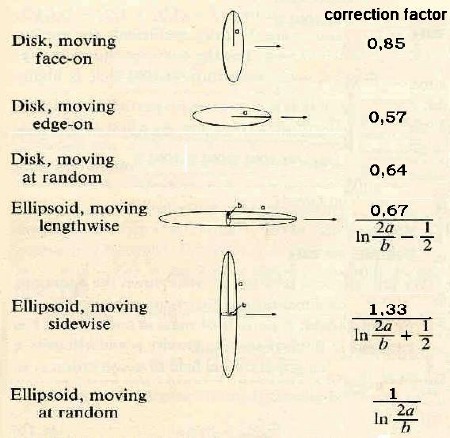
diffusion is dependent on the shape (ellipticity) of a particle. Elongated
particles are moving faster than sphe- rical ones (Perrin 1934, 1936). The
respective formulas are given by a modified copy from Berg (1993, page 57).
For randomly moving molecules with
ellipsoidal shape we have to multiply by ln(2a/b) with a as the major and b the minor axies
of the ellipsoid. Concerning DAPI the quotient a/b = 3
and ln(2a/b) = 1,8 which finally leads to
the coefficient of DAPI of being
D(DAPI) =
2,04 ● D(R6G) = 5,7 ● 10 ^-6 cm^2/sec .
DAPI migrates rapidly through its environment
Using <X^2> = 6Dt for random diffusive motion in space the
following graphs in fig. 4 demonstrate the behaviour of DAPI in aqueous
solutions to travel along paths in the nano- and micrometer scale.
Fig.4: The parabolic relationship between travel time and the respective distance covered by DAPI in aqueous solutions
Free
binding sites in native DNA – maximally 30 µm apart from the next DAPI molecule
- can be populated within 0,27 µsec, whereas the penetration of a cell nucleus
with a diameter of 5 µm and housing 6 pg DNA is done within 4 sec.
During a
typical fcm pulse of 2-5 µsec in length there is time enough for DAPI molecules to
associate with binding sites which have been released in the meanwhile.
This guarantees
the high resolution and sensitivity of DNA flow cytometric measurements.
To estimate the order of
the leaking time of DAPI from the sample core into the surrounding sheath flow
we have to apply <X^2> = 4Dt. Assuming 10 µm as the radius of the sample
core in a flow cytometer it will take about 43 seconds for the core to be
completely evacuated from DAPI molecules. This is long enough not to influence
the cytometric accuracy upon leakage of dye out of the sample stream during the
time from the formation of hydrodynamic focussing to the point of excitation
and fluorescence measurement.
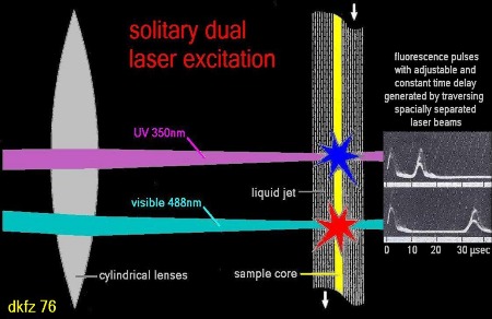
Furthermore, upon
application of the multi laser excitation mode (fig.5) with pulse delay of
about 10 to 30 µsec between sequential foci no significant degradation of the
fluorescence quality is to be expected.
Fig.5: Flow cytometry using solitary dual (or multi) laser excitation of cellular particles generates fluorescence pulses which are separated in time and have to be correlated using sample and hold electronics together with time-of-flight circuits.
In an affort to investigate photo-bleaching and photon saturation upon
high power excitation of dyes in flow Ger van den Engh and Colleen Farmer
(1992) used a dual laser cytometer with laser lines at identical wavelengths.
The first laser was tunable and served to excite the dye at different power
levels, whereas the second beam had a constant low power output to monitor the
remaining fluorescence after being bleached by the first one. Their investigations have been focussed on the behaviour of Hoechst
33258 and propidium iodide. As far as DAPI and HO-33258 have similar binding characteristics to
ds-DNA we apply the data thus obtained to our explanations of the binding
dynamics between DAPI and DNA. No declaration was given concerning the time delay between the two laser
beams. Therefore, a value is assumed around 20 µsec (fig.5). Tremendous photo-bleaching could be demonstrated with their experiment.
This can only be explained by the fact that the DNA-dye complex - despite the
dye being destroyed upon excitation -
was stable during the intersection time of 20 µsec by the two laser
beams. Otherwise released binding sites could be repopu- lated by DAPI within
0,27 µsec and bleached molecules could thus be replaced by unexhausted ones
present in the surrounding dye medium. This leads to the conclusion that the
DNA-DAPI complex does dissociate with a rather large constant rate. A
dissociation constant of 8,5/sec was observed by Tanious et al. 2008 for DAPI -
polyA-polyT complexes and this value
corresponds well with our argumentation. In conclusion, DAPI complexes with cellular DNA are
stable during the few micro- seconds of interrogation by a laser beam for
fluorescence excitation in flow. Binding sites temporarily released from a DAPI
molecule will be repopulated very fast within less than one third of a microsecond.
In conclusion:
DAPI is one of the favourites for quantitative DNA flow cytometry due to:
1. selectivity of DAPI fluorescence
(and bisbenzimidazole derivatives) to AT-rich DNA,
2. binding stability, and
3. fast diffusive replenishment of released binding sites.